Digging into Snowflake Compute Costs

Snowflake costs can be bucketed into the following categories: compute, storage, and data transfer. The compute layer consumes credits and comprises three categories: virtual warehouse compute, serverless compute, and cloud services compute. With compute spend attributing to around 80% of your total Snowflake bill, compute cost optimization is an area where all Snowflake users should be aware.

Breaking Down Snowflake Compute Costs

Resource consumption is billed via Snowflake compute credits. Credits are consumed only when resources are being used, like virtual warehouses, serverless features, or cloud services.

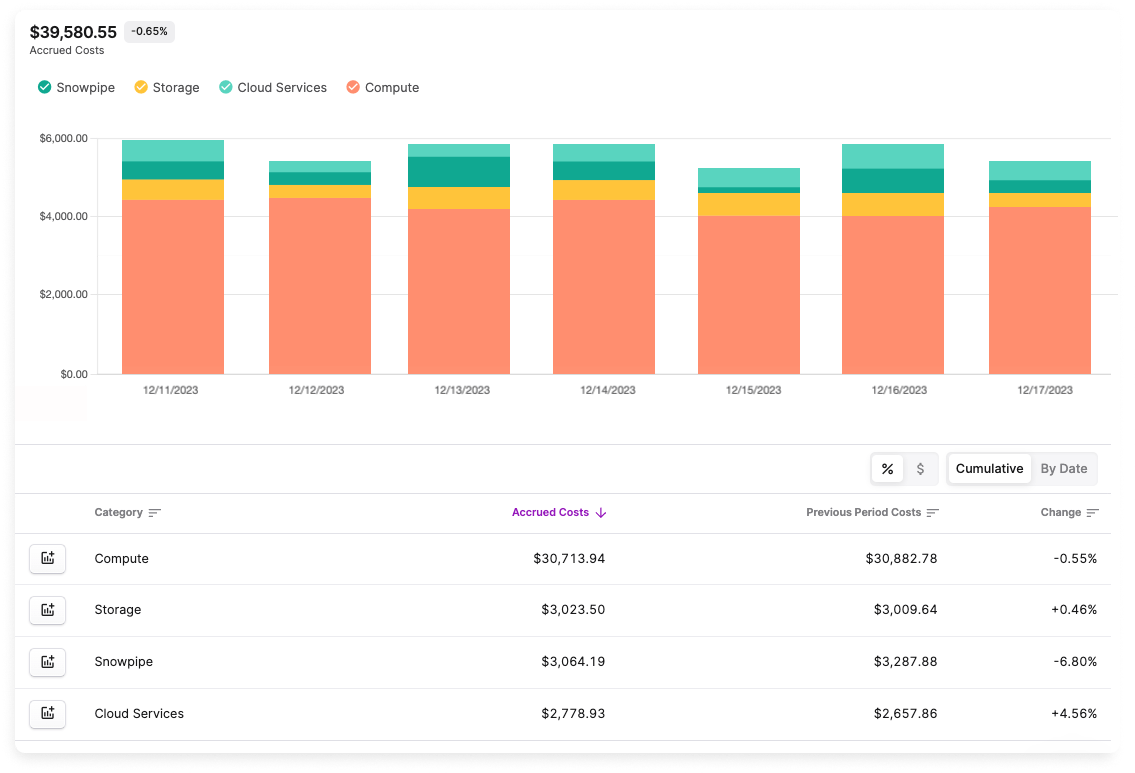
Example Breakdown of Snowflake Costs in the Vantage Console

Snowflake compute resources will consume credits based on the following factors.

Breakdown of Snowflake Compute Cost Categories

Next, we’ll dive a bit deeper into each of these categories and provide some cost optimization tips along the way.

Snowflake Virtual Warehouse Costs

Before diving into virtual warehouse costs, it’s important to understand what exactly a virtual warehouse is. At its core, a virtual warehouse is a group of computing resources (CPU, memory, etc.) that you can provision in the cloud to process and analyze data. Snowflake offers both Standard and Snowpark-optimized virtual warehouses. Snowpark-optimized warehouses provide much larger memory per node versus Standard warehouses. Warehouses can be started and stopped on demand, as well as resized, to meet any change in your requirements.

Virtual warehouse costs are based on the following factors:

• Size: Both Standard and Snowpark-optimized virtual warehouses have different warehouse sizes. For example, a Medium Standard warehouse consumes 4 credits per hour of run time, while a Medium Snowpark-optimized warehouse consumes 6 credits per hour of run time.

• Uptime: Pricing follows a consumption-based model. You pay for what you use. Warehouses that are not running do not incur charges.

• Duration: Credits are billed per second while the warehouse is running. There is a 60-second minimum charge. Note that when a warehouse is restarted, you are charged for one minute of use. (This is also true when a warehouse is resized or initially started.) Consequently, if you initiate, stop, and then restart a warehouse—all within the same minute—you will incur multiple charges as a result of the minimum charge policy.

Virtual Warehouse Cost Optimization Tips

Select the Appropriate Virtual Warehouse Size

First and foremost, always consider whether you are using the appropriate warehouse size. A Large Standard warehouse consumes 8 credits per hour of run time; whereas, a 4X-Large consumes 16 times more—or 128 credits—per hour of run time. In cases where you are constantly executing queries or have very long-running queries, consider whether a smaller warehouse size can meet your needs. The Snowflake best practice is to “start with a smaller size and slowly increase it based on workload performance.”

Set Statement Timeout

Consider adjusting the STATEMENT_TIMEOUT_IN_SECONDS parameter. The default value for this parameter is 172,800 seconds, or 2 days. This parameter can be set at the account, user, session, and individual warehouse levels, so you can specifically target instances or scenarios where you need to control long-running queries. The below example shows how to set timeout for a hypothetical warehouse. In this example, timeout is set for 3,600 seconds—or 1 hour—on a particular warehouse.

ALTER WAREHOUSE my_warehouse SET STATEMENT_TIMEOUT_IN_SECONDS = 3600;
-- timeout after 3600 seconds (1 hour)

Configure Automatic Suspension

Auto-suspension is set by default on Snowflake warehouses. This process helps minimize costs during idle periods. To optimize this feature, assess the typical duration of your queries. The default value for this parameter is 600 seconds, or 10 minutes. If your queries tend to be brief, you can potentially adjust the AUTO_SUSPEND parameter to be lower so that warehouses do not sit idle for long. This adjustment helps you to avoid unwanted compute costs during lulls in activity.

ALTER WAREHOUSE my_warehouse SET AUTO_SUSPEND = 60;
-- suspend warehouse after 60 seconds (1 minute)

Leverage Query Caching

The query cache feature is a powerful feature users can leverage to persist query results. The result cache comprises results from queries run in the past 24 hours. If a user re-runs the exact same query, within the same warehouse, Snowflake will use the already generated results rather than recomputing the query.

To leverage persisted queries, users must adhere to specific criteria. Most importantly, the second instance of the query must be exactly the same query as the first. In addition, the data in the source table cannot change between invocations of the query.

In the example below, the second line will use the query cache as it directly replicates the first instance of the query; however, the third line will not use the cache since this instance uses an alias (i.e., a) for my_table. The fourth instance uses uppercase syntax for keywords (i.e., SELECT) versus lowercase (i.e., select). Therefore, this instance of the query also does not leverage the cache, according to the query cache criteria.

select * from my_table;
select * from my_table;
select * from my_table a;
SELECT * FROM my_table;

We ran a query similar to the one below on a Medium Standard warehouse. The query returned about 6 million rows of data in 5.8 seconds. We then re-ran the exact same query, which was much quicker—145 milliseconds—as it could pull from the query cache without recomputing the results.

-- first instance of executing query
select * from my_table a
join other_table b
on a.column_1 = b.column_2
-- first query executed in 5.8 seconds

-- second instance of executing query in the same warehouse
select * from my_table a
join other_table b
on a.column_1 = b.column_2
-- second instance of query executed in 145 milliseconds

You can use the query cache to your advantage if your data does not frequently change and if you often need to re-run queries within the same timeframe. Snowflake says it best when weighing the benefits of this optimization:

…[C]onsider the trade-off between saving credits by suspending a warehouse versus maintaining the cache of data from previous queries to help with performance.

Snowflake Serverless Costs

Serverless costs come from Snowflake-managed services, such as background maintenance processes. Charges are based on the amount of time the resource runs. Snowflake uses compute-hours for serverless functions, which are calculated on a per-second basis. Total cost depends on the individual serverless feature. For example, materialized view maintenance is 10 credits per compute-hour versus query acceleration, which is 1 credit per compute-hour.

Serverless Cost Optimization Tips

Serverless cost optimization is based on the individual service. Tips for a few of these services are provided below.

Examine Materialized Views

In a previous post, we provided some best practices for using materialized views. The most important takeaway to remember when it comes to these views is that each time rows are inserted into the source table, background maintenance occurs, and the rows are inserted into the materialized view as well. Try to avoid using these views when the source data frequently changes. You’ll save on serverless background charges.

Configure Search Optimization Service

Search Optimization Service enhances performance of certain query types (e.g., substring and regular expression searches). The service prevents unnecessary micro-partitions during table scans, resulting in faster query execution. To reduce costs, carefully select the resources that use this service. If a table has a lot of data changes, more resources will be consumed and will incur greater serverless costs.

Snowflake Cloud Services Costs

Another aspect of compute billing users should be aware of is cloud services. These services include functions like authentication, displaying queries, and access control/security. The cloud services portion of the billing breakdown has its own distinct pricing structure.

You are charged for cloud services resources only after they exceed 10% of your warehouse compute credits cost. The calculation for cloud services is as follows.

Total Credits Billed = Warehouse Compute Credits Used + Cloud Services Credits Used - Adjustment for Cloud Services

The adjustment is based on whichever value is less: 10% of the warehouse compute credits used or the total cloud services credits used. The adjustment is then subtracted from the total cloud services credits and used to determine the final billing amount for cloud services on a given day. The adjustment is recalculated each day.

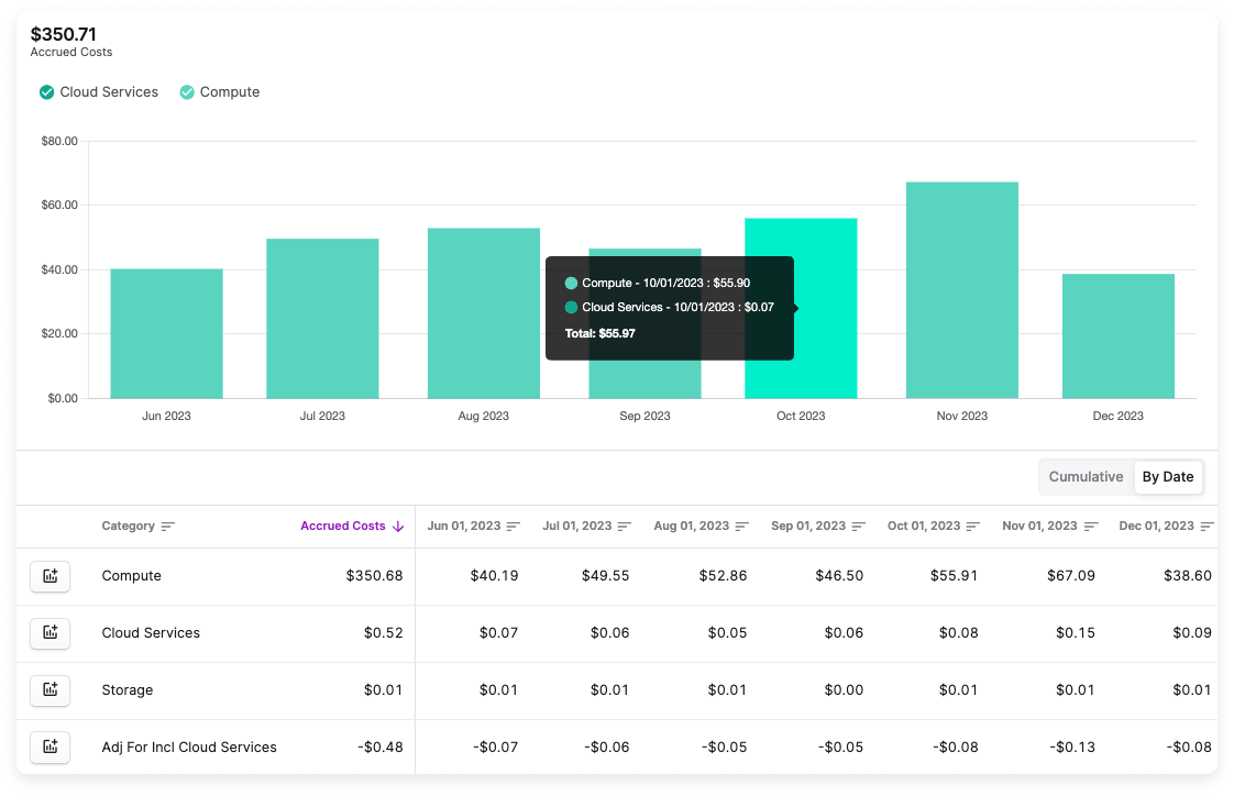
Cloud Services Costs and Adjustment in the Vantage Console

Review the below example for how this adjustment is calculated. The example demonstrates incurred charges for cloud services on three different days. Each day, the adjustment is recalculated based on the charges incurred for warehouse compute.

Example Cloud Services Cost and Adjustment

Cloud Services Cost Optimization Tips

Consider the following suggestions for reducing costs and optimizing cloud services usage below.

Avoid Full Clones

Creating full clones of databases for backups incurs significant cloud services costs. Consider cloning only a portion of the needed data, such as individual tables or columns.

Monitor Complex Queries

Complex queries with joins can use a lot of cloud services credits based on the query’s time to compile. Consider reviewing queries or monitoring cost per query to see where you may be incurring the largest costs.

Be Selective with COPY Commands

When referencing files in external locations via a COPY command, be specific on which files should be copied. Snowflake suggests structuring your source structure to include a date prefix. You can then use the optional PATTERN parameter or more easily indicate which files you want to copy from the external source.

Conclusion

While Snowflake compute often accounts for the majority of Snowflake costs, you can leverage a number of optimization techniques, including the ones presented here. With a solid understanding of what each cost represents, you can become more informed about your cost optimization practices and avoid surprising charges on your bill.